[cs224w笔记]4.网络聚类之谱分析方法

这是斯坦福cs224w的课程笔记，根据老师讲课内容、ppt和助教的笔记和自己的理解整理的。 cs224w的资源在b站和youtube都有，不过没有字幕，jure老师的口音挺可爱的，听一俩节课也习惯了，不过有时候还是配合助教的笔记看清楚一些。

助教的笔记： https://snap-stanford.github.io/cs224w-notes/network-methods/spectral-clustering

课程网站（有ppt和作业）：http://web.stanford.edu/class/cs224w/

另外， 之前没有发现原来文章的排版那么难看！稍微改了一下行距，可能会好一些orz 如果有空我会把英文部分尽量都翻译过来的

---

Spectral Clustering

Here we study the important class of spectral methods for understanding networks on a global level. By “spectral” we mean the spectrum, or eigenvalues, of matrices derived from graphs, which will give us insight into the structure of the graphs themselves. In particular, we will explore spectral clustering algorithms, which take advantage of these tools for clustering nodes in graphs.

The spectral clustering algorithms we will explore generally consist of three basic stages.

• Preprocessing: construct a matrix representation of a graph, such as the adjacency matrix (but we will explore other options)
• Decomposition: compute the eigenvectors and eigenvalues of the matrix, and use these to create a low-dimensional representation space
• Grouping: assign points to clusters based on their representation in this space

*英文内容来自助教的笔记

这一节讲的是用谱分析的方法来做网络聚类。 谱分析就是研究网络邻接矩阵的特征值和特征向量， 从而获得网络结构的一些信息。 这种方法大致分为3个步骤：

• 预处理： 构建表示图结构的矩阵，例如邻接矩阵以及laplacian矩阵。
• 分解： 计算特征值和特征向量。用它们来表示节点。
• 聚类： 将节点根据它们在representation 空间中的情况聚类。

---

Graph Partitioning

Let’s formalize the task we would like to solve. We start out with an undirected graph G(V,E). Our goal is to partition VV into two disjoint groups A,B (so A∩B=∅ and A∪B=V) in a way that maximizes the number of connections internal to the groups and minimizes the number of connections between the two groups.

To further formalize the objective, let’s introduce some terminology: 首先对问题作出定义：

• Cut: how much connection there is between two disjoint sets of nodes. cut(A,B)=∑i∈A,j∈Bwij where wij is the weight of the edge between nodes i and j. 即类A和类B之间的边的总和，如果是有权重的，就是总加权和。

  $$cut(A, B) = \sum_{i \in A, j \in B} w_{ij}$$

• Minimum cut:  使得两个部分之间联系最少的分割。

  $$argminA,Bcut(A,B)$$

Since we want to minimize the number of connections between A and B, we might decide to make the minimum cut our objective. However, we find that we end up with very unintuitive clusters this way – we can often simply set A to be a single node with very few outgoing connections, and B to be the rest of the network, to get a very small cut. What we need is a measure that also considers internal cluster connectivity.

但是仅仅考虑两个分割之间的边数是不够的，例如有一个悬挂节点，那么它和网络其他部分的边数为1, 把它作为一个类，两个类就会非常不平衡。 所以，也要考虑到聚类的内部联系。用 conductance 来衡量聚类的好坏，conductance越小，越好。

Enter the conductance, which balances between-group and within-group connectivity concerns. We define 

$$\phi(A, B) = \frac{cut(A, B)}{min(vol(A), vol(B))}$$

where

$$vol(A) = \sum_{i \in A} k_i$$

the total (weighted) degree of the nodes in A. We can roughly think of conductance as analogous to a surface area to volume ratio: the numerator is the area of the shared surface between A and B, and the denominator measures volume while trying to ensure A and B have similar volumes. Because of this nuanced measure, picking A and B to minimize the conductance results in more balanced partitions than minimizing the cut. The challenge then becomes to efficiently find a good partition, since minimizing conductance is NP-hard. 最小化conductance是一个NP-Hard问题。

---

spectral graph partitioning

1. 首先定义图的邻接矩阵A。 然后假设有一个vector x， x是所有顶点的label。 那么Ax = y ，yi的意义就是：

   节点i 的所有邻居的label的总和。

2. 特征值和特征向量的意义？ Ax = λx，意味着，有一种特殊的节点的labeling 方式，使得 我们把一个节点i的所有邻居的label加起来，作为这个节点的新label，这个label就只是原来分配的label的λ倍， 且这个倍数是对所有的节点都一样的。

Enter spectral graph partitioning, a method that will allow us to pin down the conductance using eigenvectors. We’ll start by introducing some basic techniques in spectral graph theory.

The goal of spectral graph theory is to analyze the “spectrum” of matrices representing graphs. By spectrum we mean the set Λ={λ1,…,λn} of eigenvalues λiλi of a matrix representing a graph, in order of their magnitudes, along with their corresponding eigenvalues. For example, the largest eigenvector/eigenvalue pair for the adjacency matrix of a d-regular graph is the all-ones vector x=(1,1,…,1), with eigenvalue λ=d.

可以证明， d-regular 的图中， d就是邻接矩阵最大的特征值。（1,1,…1)是它对应的唯一的特征向量。

Exercise: what are some eigenvectors for a disconnected graph with two components, each component d-regular? Note that by the spectral theorem, the adjacency matrix (which is real and symmetric) has a complete spectrum of orthogonal eigenvectors.

然后，如果是有两个连通部分，每个都是d-regular的，那么我们把一边标记为0，一边标为1， x=(0,0,..0,1,1,..1), Ax=lambdax， λ就是d。同样，也可以把一边标为1一边标为0.所以当有两个联通部分的时候， λn=λn-1. multiplicity=2（也就是λ的出现次数）。 当有k个联通部分，λn的multiplicity就是k。

What kinds of matrices can we analyze using spectral graph theory?

1. The adjacency matrix: this matrix is a good starting point due to its direct relation to graph structure. It also has the important property of being symmetric, which means that it has a complete spectrum of real-valued, orthogonal eigenvectors.A的特征向量是正交的！！！所以，xn · xn-1=0, 如果图是d-regular连通图，那么xn=(1,1,1,…), 那么xn-1的元素和必须为0.

   那么 xn-1中的元素会有一些>0, 有一些小于0！ 它就把点集分成了两半！

   

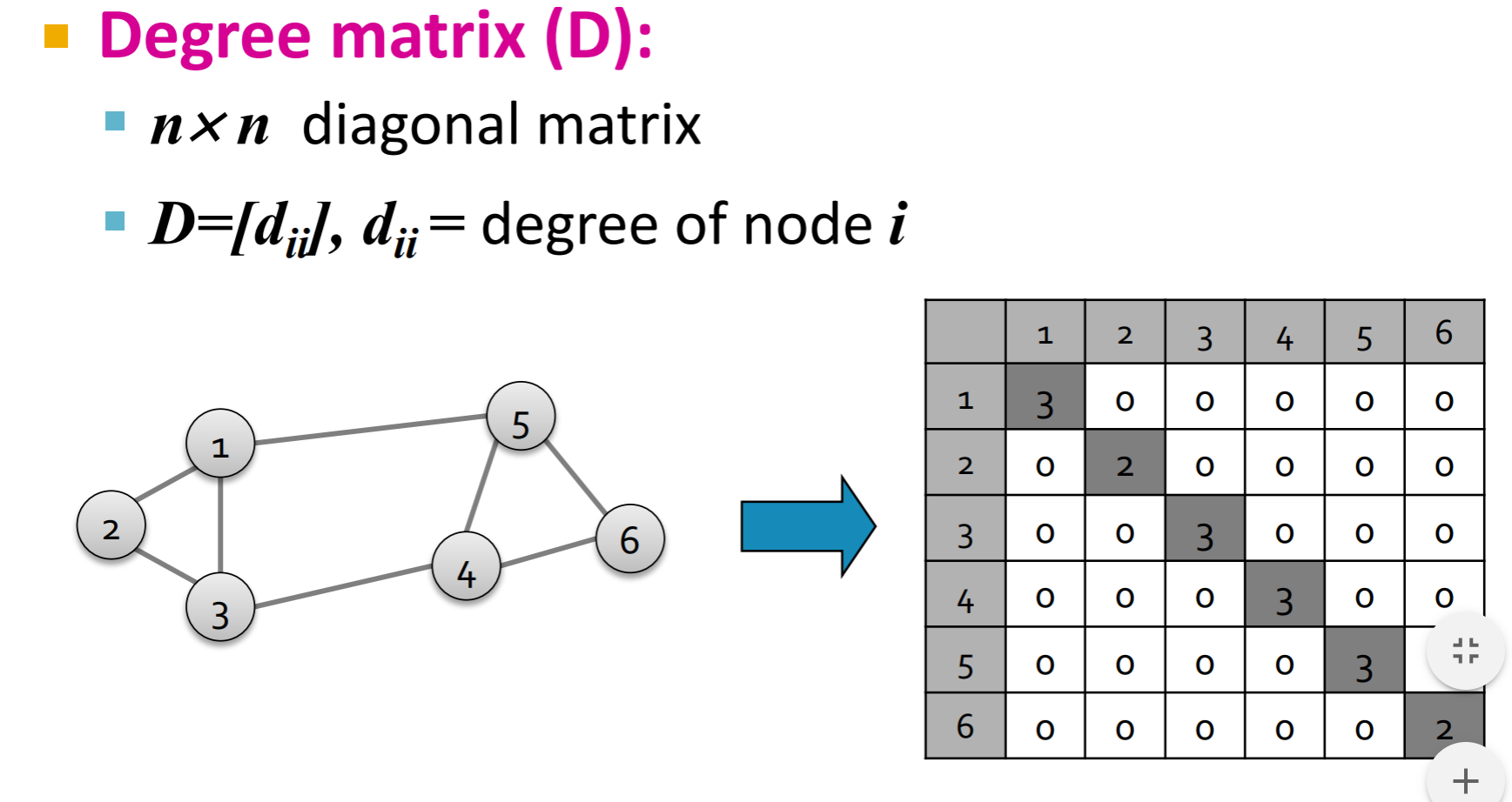
   1. Laplacian matrix ：
   $$L=D-A$$

   性质：

   1. L 的对角线是 i的度数， 而在i，j 相连的地方，Lij=-1.
   2. x=（1，1, …1） 那么 Lx=0. 所以， λ=λ1=0 最小的那个特征值是0.
   3. 那么，所有特征值都是非负的。
   4. L也是实对称阵， 那么特征向量也都是正交的，并且有n个特征值。

   In particular, λ2, the second smallest eigenvalue of L, is already fascinating and studying it will let us make big strides in understanding graph clustering. By the theory of Rayleigh quotients, we have that

   $$\lambda_2 = \min_{x: x^T w_1 = 0} \frac{x^T L x}{x^T x}$$

   where w1is the eigenvector corresponding to eigenvalue λ1; in other words, we minimize the objective in the subspace of vectors orthogonal to the first eigenvector in order to find the second eigenvector (remember that L is symmetric and thus has an orthogonal basis of eigenvalues).

   

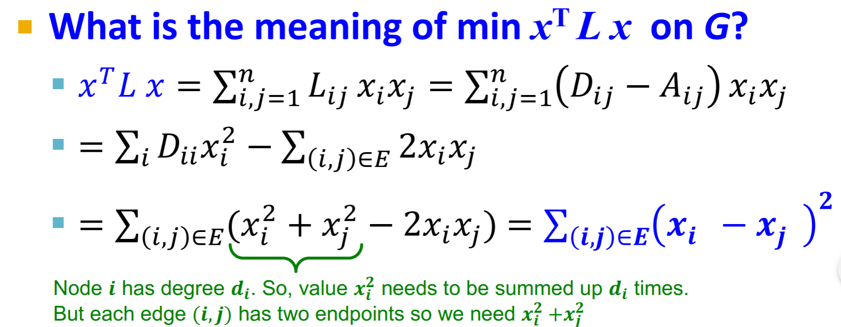
   就会变成：

   

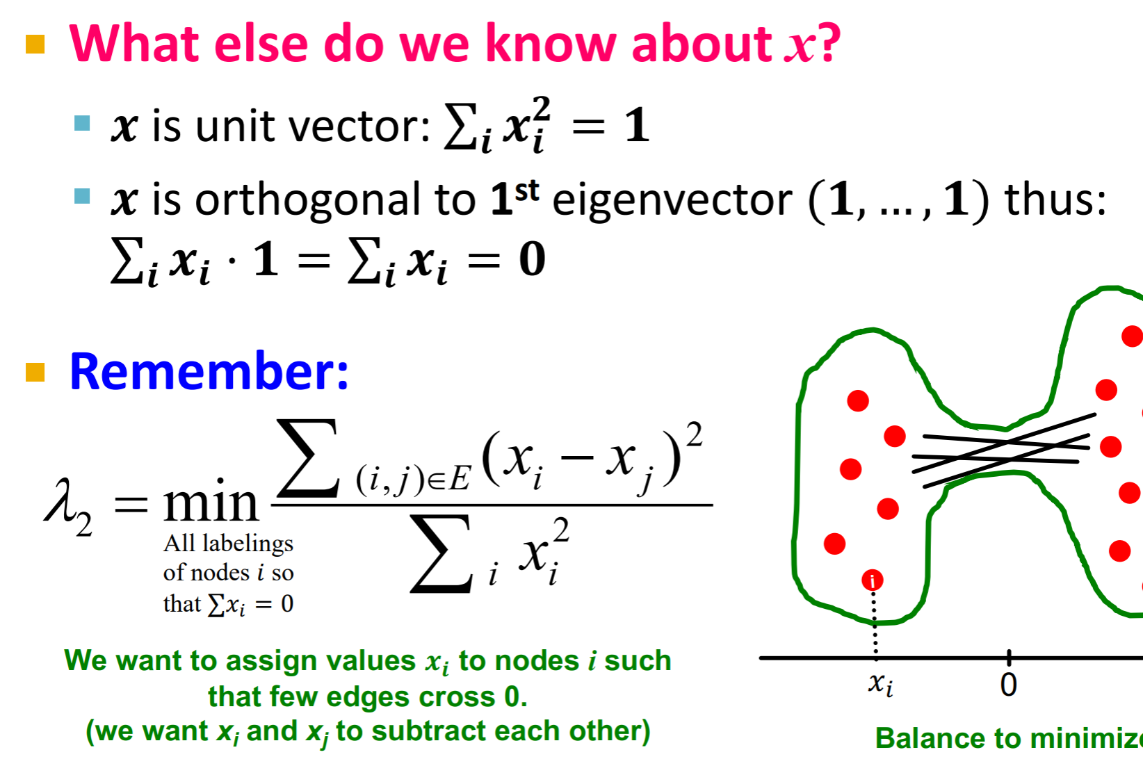
   这个目标的意义就是， xi - xj可以看作是节点i和节点j的label的距离，而当ijlabel 一个为正一个为负的时候，他们的距离平方就会大，如果是同一个分组的，平方和就会小。 那么这个式子就是在将节点分成两半，然后要横跨两个部分的边越少越好。（同一边的越多越好）

---

how to find optimal cut （Fiedler）

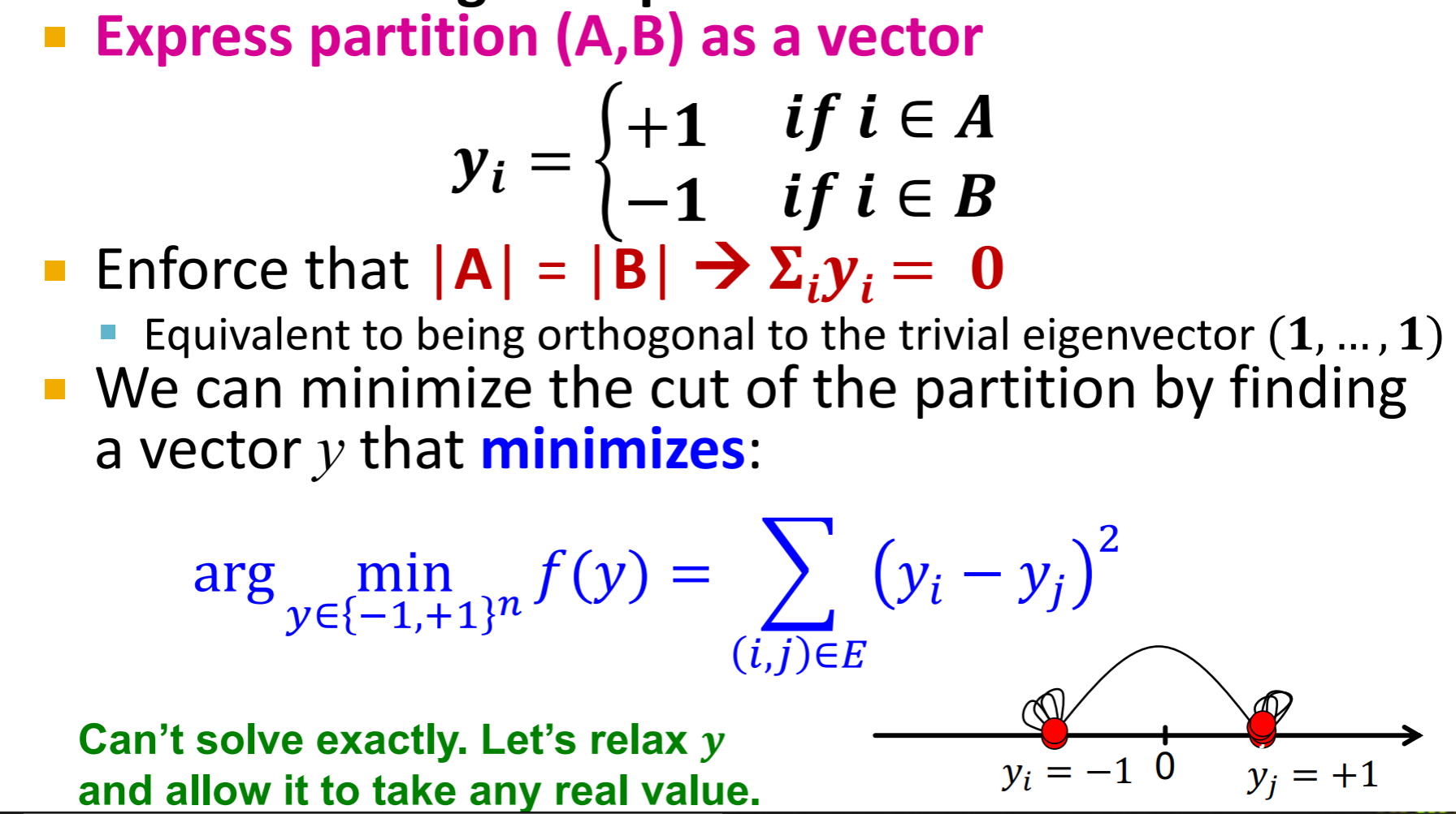
这个yi 只能取1或负1，是节点的label。这个目标实际上和λ2的目标很相似，只不过λ2那个式子里，xlabel是可以取任意实值的。但是，这个没办法求出精确解， 所以，有了下面的约束，并且让y可以取任意实值：因为和y的大小没有关系，所以可以约束

y

=1， 而

$$\sum_{i} y_{i}=0$$

就是让

A

==

B

的一个约束。

所以， λ2 = min f(y)

而， x = arg miny f(y) y的解就是λ2对应的特征向量。

Now that we have a link between an eigenvalue of L and graph partitioning, let’s push the connection further and see if we can get rid of the hard |A|=|B| constraint – maybe there is a link between the more flexible conductance measure and λ2. Let’s rephrase conductance here in the following way: if a graph Gis partitioned into A and B where |A|≤|B| , then the conductance of the cut is defined as β=cut(A,B)/|A| . A result called the Cheeger inequality links β to λ2: in particular, 

$$\frac{\beta^2}{2k_{max}} \leq \lambda_2 \leq 2\beta$$

where kmax is the maximum node degree in the graph. The upper bound on λ2 is most useful to us for graph partitioning, since we are trying to minimize the conductance; it says that λ2 gives us a good estimate of the conductance – we never overestimate it more than by a factor of 2! The corresponding eigenvector x is defined by xi=−1/a if i∈A and xj=1/b if i∈B ; the signs of the entries of x give us the partition assignments of each node. λ2可以作为分割的metrics conductance 的一个良好近似，因为λ2≤ 2β， 所以估计值比真实值大最多一倍。

---

Spectral Clustering 实做

• 算出图的Laplacian matrix L
• 计算出L 的特征值λ和特征矩阵x ， 第二小的那个λ2 对应的特征向量x2， 对应了每个节点的label
• grouping，决定x2 从哪个值分成两个partition，一般是0

---

K 个partition怎么办

• recursively cut into 2 partitions
• cluster multiple eigenvectors， 不仅是看x2， 也看x3， x4……，一个节点就会由p个值来label， 然后可以把这些在p维空间聚类。

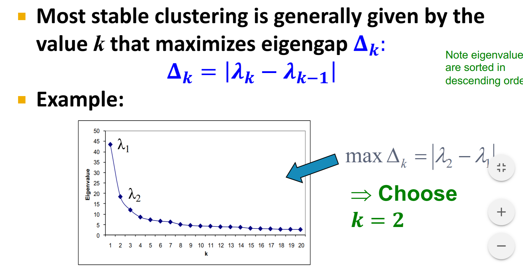
如何选择有多少个聚类？ 如何确定k？

1. eigengap： 两个相邻的特征值的绝对值差。

   Most stable clustering is generally given by the value k that maximizes eigengap Δk （这里的特征值是从大到小排序的，取从大到小扫描，两个相邻值相差最大的k）

   

---

Motif-Based Spectral Clustering

What if we want to cluster by higher-level patterns than raw edges? We can instead cluster graph motifs into “modules”. We can do everything in an analogous way. Let’s start by proposing analogous definitions for cut, volume and conductance:

1. motifs cut：cutM(S): 是一些节点在一个partition，而另一些节点在另一个partition中的motifs的数量。
2. volm(S): 是S中motif m的节点的数量。

3. motif conductance：

   $$\phi(S) = cut_M(S) / vol_M(S)$$

找到optimal cut 也一样是np-hard问题

算法：

1. preprocessing： 把原来的图转变为 一个 weighted graph，边的权重= 这条边参与motif的个数。

2. apply spectral cluster： 根据转化后的加权图，算出它的邻接矩阵A和laplacian矩阵L。 并且求L的特征值和特征向量 λ2和x2

3. grouping： 对节点按x2中的值从小到大排序， 然后分别从第i个节点处分割， 每次分割算出在第i个节点分割的motif conductance， conductance 最小的那个就是近似最好的分割。 这样比直接从0分成两半要好。

这个近似也是有可证明的保障的：

Again, we can prove a motif version of the Cheeger inequality to show that the motif conductance found by our algorithm is bounded above by 

$$4\sqrt{\phi_M^*}$$

, where 

$$\phi_M^*$$

is the optimal conductance.